Four years ago, on 23 November 2021, I published a post titled “The DART Mission,” about NASA’s attempt to crash a spacecraft into a small asteroid in an effort to divert its orbit. The launch would take place the next day, and the crash was planned on 23 September 2022. So I ended the post with: My next update about DART will probably be in October next year.
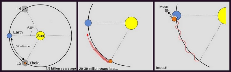
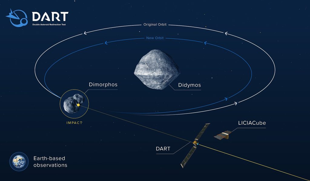
Here is finally that update ;-). Let me start with an image from that blog. Didymos is an asteroid, a Near Earth Object (NEO) and even a Potentially Hazardous Asteroid (PHA), although there is no risk of collision with Earth in the next hundred years. A tiny moonlet Dimorphos, orbits the asteroid and was the target for the mission.

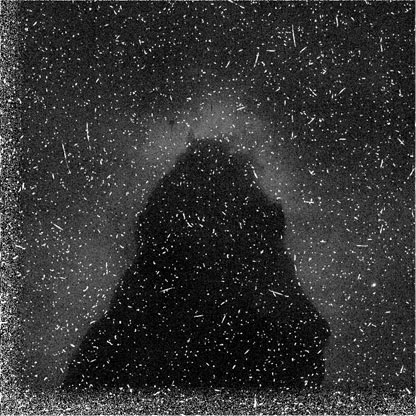
After a successful launch on 24 November 2021, DART arrived at the asteroid on 26 September 2022, about 11 million km away from Earth. How to direct DART to hit the tiny moonlet (about 150 m in diameter)? DART must do that itself with the help of its built-in camera DRACO. Four hours before reaching Dimorphos, still about 90.000 km away, DART became autonomous, using DRACO for navigation. Here is a photo taken by DRACO, 2.5 minutes before impact, the last picture where Didymos is still fully visible.

NASA collected all the pictures taken by DRACO and combined them into a time-lapse video. It shows the final 5.5 minutes, ten times faster, except for the last 6 images, which are shown in real time, every second. The “shakiness: in the beginning is a result of minor course corrections. The last image could only be transmitted partly because of the crash. A fascinating video.
The collision of DART and Dimorphos was a frontal one, so it reduced the speed of the moonlet a little but. This would cause Dimorphos to move a bit closer to Didymos with a slightly shorter period (see the first image above). Before the impact, one orbit of Dimorphos took about 12 hours. I wrote in my 2021 blog that the impact was expected to shorten the period by about 10 minutes. So it was a surprise that after the crash, the period of Dimorphos became 34 minutes shorter! In the appendix I explain how they could measure this, from Earth!
The explanation for the large reduction, was that the speed reduction of Dimorphos was not only caused by the crash of DART, but also, and even more, by the material blown away from the moonlet, causing an additional recoil.
How do we know that there was a lot of debris ejected by the crash? Because there was an eyewitness!
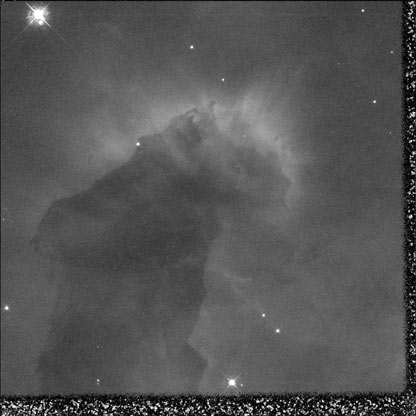
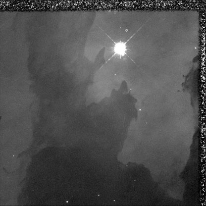
DART had on board a tiny spa craft, called LICIACub, which it released two weeks before reaching Dimorphos. This LICIACub had two cameras on board to take pictures of the crash and its aftermath. Here are two of the pictures. The left picture was taken 156 s after the impact, the right one after 175 s. The crash caused a lot of moonlet material to be ejected, probably leaving a crater in Dimorphos.

DART was very successful . It demonstrated that impacting asteroid could divert its course, important if ever an asteroid would be on a collision course with Earth.
n. October 2019 I published a blog Will an asteroid hit Earth?, after frightening reports of an impending asteroid collision with Earth appeared in the tabloid press. in that post I explained that the reports were sensational and not true. But catastrophic collisions have occurred in the past and may happen again in the future, so Earth must be prepared. NASA has its Planetary Defense program and so do other Space Agencies.,
In the context of this Planetary Defense, an ambitious collaboration started around 2013, between NASA and ESA. the Asteroid Impact and Deflection Assessment (AIDA) project. Two missions, DART by NASA and AIM (Asteroid Impact Mission) by ESA. AIM was to become the eyewitness, launched earlier than DART and going into orbit around Didymos, from where it could observe the impact and its aftermath.
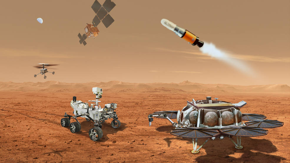
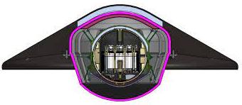
The AIDD mission is shown below. AIM (lower right) is already in orbit around Didymos and has released two CubeSats and a Mascot lander which is hovering at the moonlet, here still called Didy-moon.

A fascinating project. But already a few years later, in 2016, ESA had to cancel the AIM mission, because Germany was unable/unwilling to contribute its portion of the funding. NASA decided to proceed with DART anyway and managed to include inro the spacecraft a CubeSat, which could act as an eyewitness. In my blog about DART, I wrote: As an European, I feel rather ashamed.
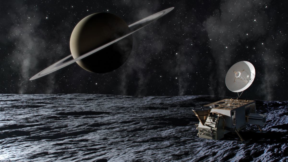
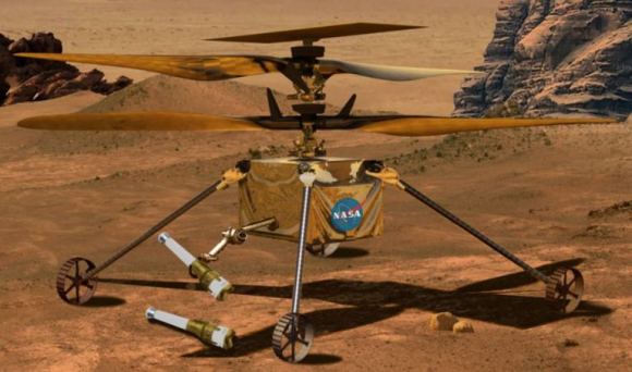
Then, in 2018, ESA came up with an alternative for AIM, called Hera. Basically, with the same mission, only reaching the asteroid in 2026, four years after the impact of DART. Here is an artist’s impression. It shows Dimorphos, with a very pronounced crater, the result of the crash. Two CubeSats are shown. No lander, but one if the CubeSats may land on the moonlet at the end of the mission.

Hera was successfully launched on 7 October 2024 and is now on its way to Didymos, where it will arrive in late 2026. In 2022 The atseroid was 11 million km away from Earth, but Hera has to travel nuch farther, abou 190 miilion km. In the video you can follow the trajectory of Hera. On12 March 2025 the spacecraft has used a gravity assist from Mars to get the right course to Didymos. In the vidoe Hera is the orange dot and Didymos the red one.
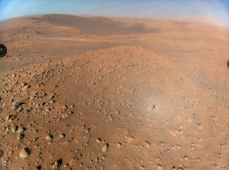
During the flyby Hera took fascinating pictures of Mars and its small moon Deinos.

When Hera arrives at Didymos, it will go into orbit around the binary asteroid. Spacecraft has landed on asteroids and crashed into them, but never gone into orbit. It needs careful navigation, much of it autonomous. Hera will study the crater formed by the impact of DART and investigate the properties of Didimos and Dimorphos. A fuill programme for the planned 6 months of the mission.

Appendix
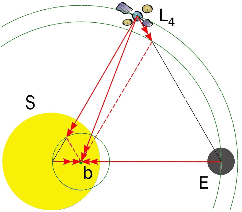
You may wonder how astronomers discovered that Didymos had a companion, the tiny moonlet Dimorphos. Even with large telescopes, the asteroid shows as a tiny speck of (reflected) sunlight. In 2003 scientists noticed that the brightness of the speck of light varied periodically, showing tiny dips. They concluded that there had to be a companion transiting the asteroid, passing in front and at the back! They could measure the period to be 11 hours and 55 minutes, before the impact, and 34 minutes shorter after the impact.+
This image shows the effect, in an exaggerated way. The big dips are when Dimorphos passes behind the asteroid, the smaller ones when it transits before the ateroid, blocking a bit of its light.

The actual effect is so small that the scientists need advanced techniques to filter the data.